Quantization explained, like you are five.
In the era of extravagence, where models casually cross 100B parameters, devouring over 500GB of GPU memory and costing millions of dollars for a single training session, quantization comes in as a prudent accountant.It ensures that models refrain from indulging in excessive memory consumption while minimizing any loss in model quality. In this blog post, we aim to demystify this potent mathematical framework using intuitive explanations, relatable examples, and accessible language. We will also delve into the fancy jargons and the ugly math that come along with quantization, just deeply enough to allow readers to nagivate research papers and documentation on quantization libraries. The objective is to make these esoteric concepts more approachable and less daunting. So buckle up as we embark on this journey, as we learn how to take mammoth ML models, and prune them down to preserve only the essential.

Why bother learning about Quantization?
In recent years, both language models and computer vision models have undergone a significant evolution, with newer models boasting unprecedented sizes and complexities. For instance, language models like GPT-3 and computer vision models like EfficientNet have reached staggering parameter counts, with GPT-3 having 175 billion parameters and EfficientNet surpassing billions of parameters across its variants.
However, the sheer size of these models presents practical challenges, particularly in terms of deployment on everyday devices. Consider a language model like GPT-3—its inference alone demands extensive computational resources, with estimates suggesting the need for multiple high-performance GPUs. Similarly, for computer vision tasks, deploying models like EfficientNet on resource-constrained devices can be daunting due to their computational and memory requirements.
To overcome these hurdles, techniques such as quantization have emerged as indispensable tools. By compressing the parameters of these large models into lower precision formats, such as INT8, quantization offers a pathway to significantly reduce memory footprint and computational demands without compromising performance. This is crucial for making these cutting-edge models accessible and deployable across a diverse range of devices, from smartphones to edge devices.
To summarize, learning about quantization, will help you deploy large models, on relatively small devices, while also consuming less power. But before we delve into the core quantization concepts, let us first look at the common data types used in Machine Learning.
0. Common Data Types in Machine Learning
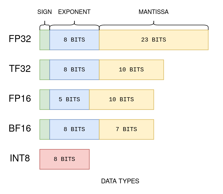
In machine learning, data types, or precision, play a vital role in model performance and efficiency. The most common data types used include float32, float16, bfloat16, and int8.
-
Float32 (FP32): This 32-bit floating point representation offers a wide range of numbers, with 8 bits for the exponent, 23 bits for the mantissa, and 1 bit for the sign. FP32 provides high precision and dynamic range suitable for most computations.
-
Float16 (FP16): With 5 bits for the exponent and 10 bits for the mantissa, FP16 offers lower precision compared to FP32. While efficient for many computations, FP16’s limited dynamic range can lead to overflow and underflow issues.
-
Bfloat16 (BF16): BF16 addresses the limitations of FP16 by allocating 8 bits for the exponent and 7 bits for the fraction. This allows it to maintain the dynamic range of FP32 while sacrificing some precision.
-
Int8 (INT8): Int8 consists of an 8-bit representation capable of storing 2^8 different values. While it offers lower precision than floating point formats, INT8 is often used in quantization to reduce model size and improve inference efficiency.
In the context of quantization, FP32 is considered full precision, while FP16, BF16, and INT8 are referred to as reduced precision formats. During training, a mixed precision approach may be employed, where FP32 weights are used as a reference, while computations are performed in lower precision formats to enhance training speed and resource efficiency. This allows for efficient utilization of computational resources while maintaining model accuracy.
1. What is Quantization?
Quantization, simply put, is the art of converting all decimal numbers ( ex. float32) in your data, into whole numbers within a fixed range (ex. int8), with a mathematical framework, that still allows us to recover the original decimal number from the whole number when needed. This is ofcourse an oversimplicatoin, if there ever was one. While the description might seem straightforward, quantization is more of an art than a rigid science. The conversion methodology is not set in stone and lacks strict determinism, which is what makes it fun, and blog worthy.
Let’s envision a scenario where we have a full HD image of a cat, occupying a hefty 8 megabytes of memory. Now, through the magic of quantization, we pixelate this image just enough to lose some fine details while retaining the essence of the feline subject. As a result, the memory storage required to represent the image diminishes significantly, perhaps to just a fraction of its original size. This trade-off between fidelity and memory efficiency encapsulates the essence of quantization, where the reduction in granularity leads to tangible benefits in terms of resource optimization. Just as pixelation preserves the overall identity of the cat in our image, quantization ensures that our deep learning models maintain their performance while operating within constrained memory environments.
2. Fundamentals of Quantization
Before we get into the ugly math and fancy jarons, let us understand the intuition. Quantization (however fancy it may sound) is just converting decimal values ( eg. float32 ) into whole numbers (eg. int8 ), in a way that it is feasible to recover the decimal number back from the whole number. Lets say we want to quantize a list of float values that are all between -4.0 and +4.0. And we want to represnet these float values in a universe that just consists of integers between -127 and 127. We would like to have a mechanism, wherein, the minimum value -4.0 maps to -127, and the maximum value +4.0, maps to 127. This would allow us to caputure the essence of all the float values in this only-integer universe of ours. Let us understand how we quantize our list of decimal values, one step at a time.
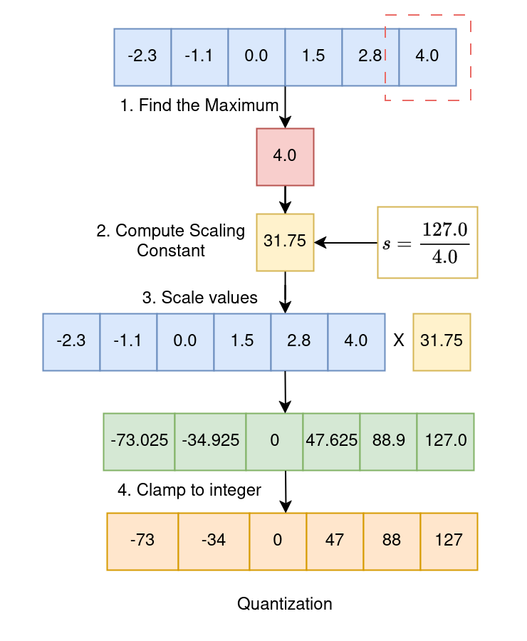
Original float array to be quantized :
[-2.3, -1.1, 0.0, 1.5, 2.8, 4.0]

STEP 1 : Find the maximum value in the array
max([-2.3, -1.1, 0.0, 1.5, 2.8, 4.0]) = 4.0

STEP 2 : Calculate the scaling constant
s = 127/4.0 = 31.75

STEP 3 : Multiply all values in array by scaling constant
=  [-2.3, -1.1, 0.0, 1.5, 2.8, 4.0] * 31.75
=  [ -73.025, -34.925, 0, 47.625, 88.9, 127.0]

STEP 4 : Round all numbers to obtain integer representation.
         Clamp all numbers between (-127,127)
= [-73, -35, 0, 47, 127]                    <---- Quantized Values
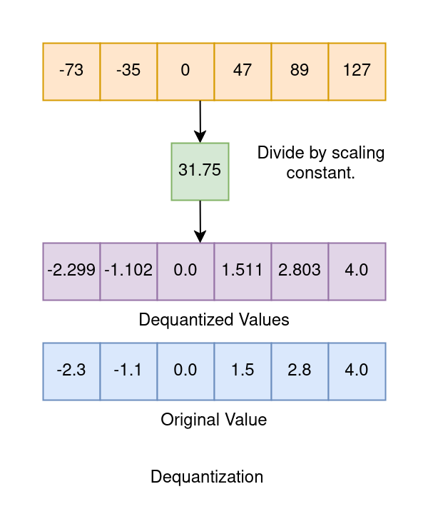
Dequantization for recovering original values :

STEP 5 : Recover original number by dividing by scaling constant.
= [-2.299, -1.1023, 0, 1.5118, 2.8031, 4.0] <---- Dequantized Values
As we can see, after division by scaling constant, we were able to reasonably approximate the orignal float values from the quantized value. We will refer to STEP 3 and STEP 4 as Quantization and STEP 5 as Dequantization.
Okay, now as promised, presenting the same ideas explained above, but with the ugly math and fancy jargons. The fancy jargons, we shall now deal with include :
- Range Mapping
- Scale Quantization
- Affine Quantization
- Tensor Quantization Granularity
- Per Tensor Granularity
- Per Element Granularity.
- Per Row/Column/Channel Granularity
- Calibration
Lets understand them one at a time.
2.1 Range Mapping
Range mapping, as the names suggest, is the mechanism for transforming continuous float values into discrete integers. Let’s denote the chosen range of representable real values as \([\beta, \alpha]\), similar to -4 and +4 in earlier example. Let the signed integer space be restricted to the bit-width b. In earlier example, since the signed integer universe had range of {-128,127}, the bit width was 8. The process of quantization involves mapping an input value \(x ∈ [β, α]\) to reside within the range \([−2^{b-1}, 2^{b-1} - 1]\). This mapping can either be an affine transformation \(f(x) = s.x + z\) or, its special case \(f(x) = s.x\) where \(x, s, z ∈ R\). We refer to these mappins as affine mapping and scale mapping respectively.
2.1.1 Affine Mapping
This mapping usually takes place using multiplication (scaling) with a scaling factor s, \(f (x) = s · x\). Another variant of this mapping can be affine mapping. Affine mapping, is just scaling, along with addition of a constant called zero point \(z\), \(f(x) = s · x + z\). The constant in affine mapping \(z\) is called zero point because it represents the value in the quantized integer space, that corresponds to the zero in the float space. Now, let’s delve into the math that underlies these transformations and understand how they bring about the crucial conversion from continuous to discrete representations.
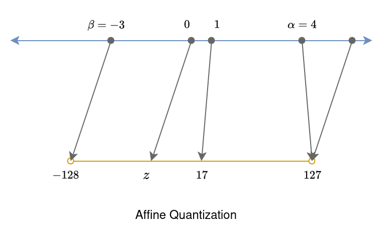
Affine quantization serves as the bridge that maps a real value \(x \in \mathbb{R}\) to a \(b\)-bit signed integer \(x_p \in \{-2^{(n-1)}, -2^{(n-1)} + 1, ..., 2^{(n-1)} - 1\}\). The transformation function \(f(x) = s \cdot x + z\) is defined by:
\[s = \frac{2^{(b - 1)}}{\alpha - \beta}\] \[z = - \text{round}(\beta \cdot s) - 2^{(b-1)}\]Here, \(s\) is the scale factor, and \(z\) is the zero-point - the integer value to which the real value zero is mapped. For an 8-bit representation \(b = 8\), \(s = \frac{255}{\alpha - \beta}\) and \(z = - \text{round}(\beta \cdot s) - 128\). The quantize operation, described by the equations below, involves clipping the result to the specified range:
\[x_p = \text{quantize}(x, b, s, z) = \text{clip}(\text{round}(s \cdot x + z), -2^{(b-1)}, 2^{(b-1)} - 1)\]The dequantize function provides an approximation of the original real-valued input \(x\):
\[x̂ = \text{dequantize}(x_p, s, z) = \frac{1}{s} (x_p - z)\]This transformation ensures the mapping of real values to int8 representation with affine quantization, where \(s\) represents the ratio of the integer-representable range to the chosen real range.
2.1.2 Scale Mapping
Scale quantization performs range mapping with only a scale transformation, using multiplication (scaling) with a scaling factor s, \(f (x) = s · x\). We focus on the symmetric variant of scale quantization, where the input range and integer range are symmetric around zero. In this case, for int8, the integer range is {−127, 127}, avoiding the value -128 in favor of symmetry. Here, the zero point in the float space, maps to the zero point in the integer space.
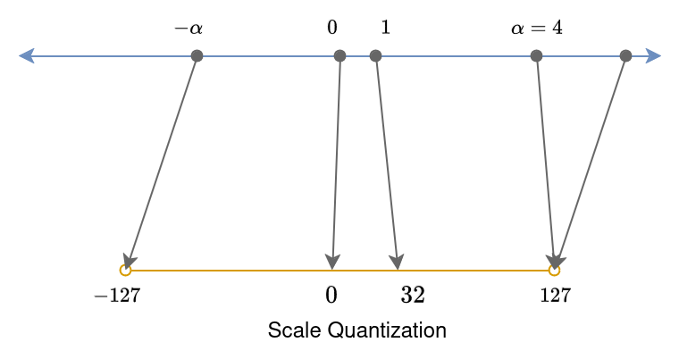
We define the scale quantization of a real value \(x\), with a chosen representable range \([−α, α]\), producing a \(b\)-bit integer value, \(x_q\) as follows,
\[s=\frac{2^{b−1}−1}{α}\] \[x_q=quantize(x,b,s)=clip(round(s⋅x),−2^{b−1}+1,2^{b−1}−1)\]We recover the approximate original value using the dequantize operation for scale quantization as follows.
\[x̂=dequantize(x_q,s) = \frac{1}{s}{x_q}\]The scale mapping is similar to the example we looked at earlier, where we quantize by multiplying with a constant, and dequantize by dividing with the same constant.
2.2 Quantization Granularity
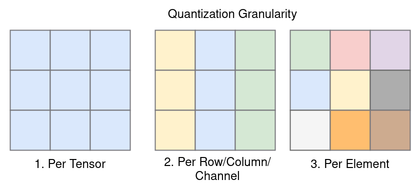
The scaling factor \(s,z\) are referred to as quantization parameters. The effectiveness of quantization, is entirely dependent of the choice of these parameters. While performing quantization for a neural network graph, we want to quantize the inputs tensors, ( activations ) and also the corresponding weights before performing the operation. The term quantization granularity refers to the level at which quantization parameters are shared among tensor elements. Here are the common choices for quantization granularity:
-
Per Tensor Granularity: In this approach, the same quantization parameters are shared by all elements in the entire tensor. It is the coarsest granularity and implies that the entire tensor is treated as a single entity during quantization and all elements have the same scaling factor \(s\) and zero point \(z\).
-
Per Element Granularity: At the finest granularity, each element in the tensor has its individual quantization parameters. This means that each element is quantized independently.
-
Per Row/Column/Channel Granularity: For 2D matrices or 3D tensors (like images), quantization parameters can be shared over various dimensions. For example, quantization parameters may be shared per row or per column in 2D matrices, or per channel in 3D tensors.
The choice of quantization granularity affects how quantization parameters are applied to the elements of the tensor, and it provides flexibility in adapting quantization to different structures within the data. Here is a general rule guide for choice of granularity.
-
Weights : Use per column granularity for weights tensor. All elements in a column of weights tensor should have same quantization parameters.
-
Activations/Inputs : Use per tensor granularity for activations or inputs to the network. All elements of the entire input tensor should have same quantization paramters.
2.3 Calibration
Quantization, as we’ve learned, is the process of converting continuous numerical values into a discrete representation. Calibration, in this context, is the art of carefully choosing the parameters that guide this conversion. Let’s dive into the intuition behind calibration before exploring three calibration methods.
In the quantization process, we aim to squeeze a broad spectrum of real-numbered values into a limited integer space. Calibration ensures we choose the right boundaries for this squeeze, allowing us to maintain the essence of our data while mapping it to a more compact form. Think of it as finding the sweet spot that captures the diversity of values in our model without losing critical information.
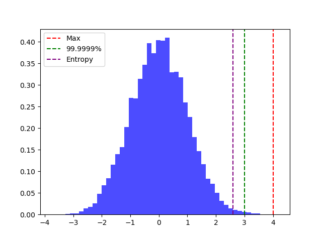
There are three major strategies to find the correct quantization paramters given the distribution of the values being quantized :
-
Max Calibration: Simple yet effective, this method sets the range based on the maximum absolute value observed during calibration. It’s like saying, “Let’s make sure we cover the extremes.”
-
Entropy Calibration: This method leverages KL divergence to minimize information loss between original floating-point values and their quantized counterparts. It’s a nuanced approach, aiming to preserve the distribution of information.
-
Percentile Calibration: Tailored to the data distribution, this method involves setting the range to a percentile of the absolute values seen during calibration. For instance, a 99% calibration clips the largest 1% of magnitude values.
Each method brings its own flavor to the calibration process, ensuring that the quantized model not only fits the data but also does so intelligently, preserving crucial details. Calibration becomes the bridge that connects the continuous world of real numbers to the discrete universe of quantization.
3. Conclusion
In conclusion, we’ve explored the fundamentals of quantization, ranging from simple examples of quantization and dequantization to more advanced topics such as range mapping, tensor quantization granularity, and calibration. By delving into concepts like scale quantization, affine quantization, and different granularities of tensor quantization, we’ve gained a deeper understanding of how quantization optimizes model memory and computational efficiency without sacrificing performance. In the next blog post, we’ll dive into concrete Python and PyTorch examples to illustrate how these concepts translate into practice, empowering readers to implement quantization techniques effectively in their machine learning workflows. Stay tuned as we continue our journey into the realm of quantization and its transformative impact on machine learning models.
Enjoy Reading This Article?
Here are some more articles you might like to read next: